These GNSS-IR use cases are selected from various GNSS archives around the world to give you examples of successful GNSS-IR. The daily solutions are generated for stations where one would expect to use the daily average reflector height. The subdaily use cases present multi-GNSS results as a function of time.

General Principles

The goal of this web app is to measure the vertical distance (or reflector height RH) between the GNSS antenna and the horizontal surface (snow, water, soil moisture, soil) below the antenna. If you are familiar with the method and want to try out the technique at different places, choose one of the sites in examples above. The API will retrieve the GNSS data and orbits from an archive, extract the SNR data, estimate reflector height and display the results.

The main idea behind the GNSS-IR technique is shown for a single GNSS signal. If a surface below a GNSS antenna is fairly planar(smooth), the reflected signal will be observed by the GNSS system. This effect is especially prominent at low satellite elevation angles. Each rising or setting satellite arc can potentially be used, which allows subdaily RH to be estimated if desired.

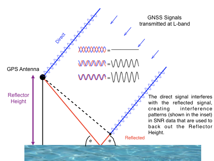
The direct signal (blue) interferes with the reflected signal (red) creating interference patterns that change over time. It is these changes (constructive and destructive) in the interference pattern that are used to estimate the Reflector Height (RH). Sample interference patterns are provided in the center of the figure.

What do the data look like? Below we highlight the raw SNR observation data for a single satellite rising arc at a typical geodetic station in Boulder Colorado ( p041). The units of the Signal to Noise Ratio (SNR) data have been changed from their native db-Hz values to a linear scale (volts/volts) and detrended, leaving only the decaying sinusoid. It is the frequency of that decaying sinusoid we want, because it tells us the Reflector Height.

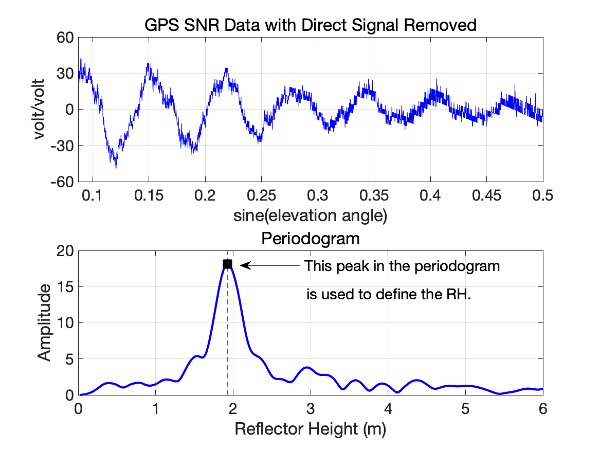
You can extract the frequency of this sinusoid using a variety of techniques, but what we have done is use the Lomb Scargle Periodogram. This technique is mainly used when the observations are not evenly sampled.

We find where the periodogram has the highest amplitude, and the RH associated with that amplitude is the estimated RH. However, we cannot assume this is a significant peak. There are a lot of different ways to assess whether a spectral peak is significant. The gnssrefl software and this webapp uses two: (1)the required amplitude of the peak and/or (2) how large the peak is relative to the periodogram values for a given RH range (i.e. 0.5 to 6 meters in this example).

The antenna phase center for p041 is a little bit less than 2 meters above the soil. (The surface is not completely smooth however). If we use the reflection zones tab on this website, we can get an idea of what the reflection zone looks like. Each colored ellipse represents a single rising (or setting) GPS satellite arc. There are five colors because five different elevation angles are shown (5,10,15,20,25). The estimated RH will be based on the data from these reflection zones.

---

Output

Now to the gnss-reflections web app. It returns two plots and a list of RH (in either plain txt or csv format). The first plot is a geographic view of the reflector height retrievals (southeast, southwest, and so on). Colors mean it is a successful retrieval and gray is unsuccessful). Reflector Height is on the x-axis.

The second plot takes the results from the previous plot and summarizes then with azimuth (degrees) on the x-axis. The top plot has Reflector Height (meters) on the y-axis. Blue means the retrieval passed QC. The second and third plots tell you how these retrievals were "scored" on the two QC parameters.

Please note that the API returns the numerical results in a plain text file.

We have put together a large number of use cases to give newcomers some feel for how the technique works. These are meant to be used with the desktop gnssrefl software.